R Speed with Ease

R vectorized

Typically, to solve this problem in R you would dip into vectorized solutions, perhaps using indexing, base R’s ifelse(), or fifelse() from {data.table}. The drawback to the latter instances in this particular use-case are they may produce warnings, which we will suppress later.

# Indexing
r_vec <- function(x) {
    out <- vector('double', length(x))
    idx <- x > 0
    
    out[idx] <- sqrt(x[idx])
    out[!idx] <- sqrt(x[!idx]^2)
    out
}

# Base R ifelse
r_ifelse <- function(x) {
  ifelse(x > 0, sqrt(x), sqrt(x^2))
}

# {data.table} equivalent of ifelse but faster
r_fifelse <- function(x) {
  data.table::fifelse(x > 0, sqrt(x), sqrt(x^2))
}

R loops

Perhaps, your brain works better using for loops. In base R this can be achieved quite simply by allocating a new vector and injecting the modified values.

# Slow R loop
r_loop <- function(x) {
    out <- vector('double', length(x))
    
    for(i in seq_along(x)) {
        if(x[i] > 0) {
            out[i] <- sqrt(x[i])
        } else {
            out[i] <- sqrt(x[i]^2)
        }
    }
    return(out)
}

Rcpp

Now we leverage {Rcpp} via cppFunction() to return a function named rcpp_loop. If you squint, you will see this looks very similar to the for loop from base R. The number of lines of code is also very similar. There are however a couple main differences of note:

• Indexing starts at 0, not 1
• Data requires a declared type (e.g. NumericVector)
• Semicolons (;) must be used as a line terminator

# Using C++ via Rcpp (function name: rcpp_loop)
Rcpp::cppFunction("
NumericVector rcpp_loop(NumericVector x) {

    int n = x.size(); // Size of input vector
    NumericVector out(n); // Create blank vector of equal size
    
    for(int i = 0; i < n; i++) {
        if(x[i] > 0) {
            out[i] = sqrt(x[i]);
        } else {
            out[i] = sqrt(pow(x[i], 2.0));
        }
    }
    return out;
}")

Comparison

To compare the various functions, we generate a vector of 100,000 numbers from -500 to 500. To ensure all the functions return the same values, we pass this vector into each function and compare the results. For speed comparisons, we run microbenchmark 250 times for each function.

# Test data
my_vec <- runif(1e5, -500, 500)

# Check equality (returns content if all equal)
check_eq <- Reduce(\(x, y) if(all.equal(x, y)) x else FALSE,
                   x = list(rcpp_loop(my_vec),
                            r_vec(my_vec),
                            suppressWarnings(r_ifelse(my_vec)),
                            suppressWarnings(r_fifelse(my_vec)),
                            r_loop(my_vec))
                   )

# Benchmark
cpp_benchmark <- microbenchmark(rcpp = rcpp_loop(my_vec),
                                r_ifelse = suppressWarnings(r_ifelse(my_vec)),
                                r_fifelse = suppressWarnings(r_fifelse(my_vec)),
                                r_vec = r_vec(my_vec),
                                r_loop = r_loop(my_vec),
                                times = 250)

# Output results
print(cpp_benchmark, order = 'median')

## Unit: microseconds
##       expr    min     lq      mean  median     uq     max neval
##       rcpp  421.0  445.3  541.5432  474.65  525.5  4442.3   250
##  r_fifelse 1712.2 1867.1 2265.2816 1974.15 2152.8  7827.6   250
##      r_vec 2079.3 2268.6 3243.7660 2617.30 2919.8 55034.8   250
##   r_ifelse 2904.2 3174.9 4144.4700 3744.00 4076.6  9514.2   250
##     r_loop 7694.0 7819.9 7956.5692 7893.70 7981.9 10615.7   250

When sorted by the median run time across replications for each function we get a range from ~500 microseconds to ~8000 microseconds. Although the table is nice, it is easier to see the differences between replications and each function when presented in a plot.

boxplot(cpp_benchmark, log = TRUE, outline = TRUE)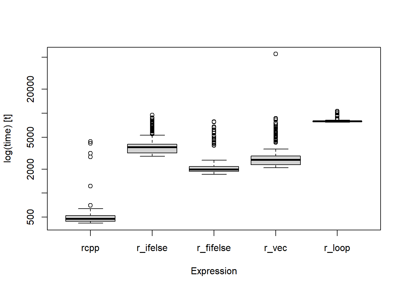

Figure 1: Comparison of different functions and their run times (logged microseconds) across 250 replications.

The {Rcpp} coded for loop was the fastest, the vectorized R function and datatable::fifelse() performed similarly, and the base R loop performed the worst overall (on my system anyway!). Using {Rcpp} can definitely make code run quickly, perhaps almost as quick as this dog…