Bayes' Town: A place of data simulation
Welcome to Bayes’ Town
Bayes’ Town is a special place, a place where we can be omnipotent and omniscient. We take comfort in having knowledge and control of all things, even though we know the entire place is apart from reality, a muddled reflection at best and a complete fantasy at worst. Bayes’ Town is a simulation, a useful tool to explore scenarios and test hypotheses, based in reality or otherwise.
For public health, creating a synthetic population can be a valuable tool. Population characteristics, and relations between them, can be modeled based upon prior knowledge or to understand ‘what-if’ scenarios. Sometimes, it even is just a good way to better understand how a model is working. If you know the generative process of a synthetic population then you can see how well certain models perform under those circumstances. More on this later…
Simulating Bayes’ Town’s Blight
As we are the masters of our simulated domain, we can decide exactly how the characteristics of our Bayes’ Town citizens are connected. Citizens of Bayes’ Town are very concerned about disease, specifically the rampant Disease X. Fortunately for us, as the creators we can instantly summon the image of how the population is impacted by this pestilence. We can visualize the relationship as a network between variables of sex, age, and whether or not the individual lives in an urban or rural location. Using DiagrammeR and the DOT language, we can visualize this relationship.
Figure 1: The “known” relationship between Disease X and the citizens of Bayes’ Town.
Generate Bayes’ Town
With this knowledge we can generate data on our citizens for this particular scenario. The core functionality is powered by rJAGS but to make it a bit easier to use, the process is wrapped up into an R6 object called BayesTown. This should be familiar to anyone from object-orientated programming (OOP) languages like Python but perhaps a bit foreign for those more comfortable with multiple dispatch, which is the common approach in R (S3 and S4) and Julia. To create a population of 1,000 people we provide some predefined information to the new (construct) method. The inputParam and simModel values will be discussed later in the methodology section.
newTown <- BayesTown$new(population_size = 1000,
                      jags_data = inputParam,
                      n.chains = 2,
                      n.iter = 5000,
                      jags_model = simModel)
The output provides some basic information on the model graph and a snapshot of the data sample. This includes all the information from the simulation, including the various data variables, coefficients, and distribution parameters. Due to sampling variation, subsequent runs with the same parameters will create slightly different populations.
Explore simulated population
To explore the simulated data, we extract the variables we observed in the diagram above. This is easily done by method chaining set_variables (to sample only particular variables/parameters) and resample (to rerun the simulation).
# Import library for some exploration work
library(dplyr)
library(magrittr)

# Data sample just to include the set of variables in the list
newTown$set_variables(c('age', 'sex', 'urbanRural', 'disease'), mode = 'include')$resample()

# Output first 5 rows of simulated data
head(newTown$data, 5)

# Summarize some basic information using dplyr
newTown$data %>%
  group_by(sex, urbanRural) %>%
  summarise(meanAge = mean(age),
            diseasePerc = 100 * (sum(disease)/nrow(.)))
Here is a sample of the simulated data:
##         age disease sex urbanRural
## 1  24.43352       1   0          1
## 2  22.56561       0   1          1
## 3  28.10493       0   1          1
## 4  33.43865       0   0          1
## 5  37.12840       0   1          1
## 6  56.35582       1   1          1
## 7  37.24761       0   1          1
## 8  47.65436       0   0          0
## 9  30.83504       0   1          1
## 10 33.03936       0   0          1
And here are some summary statistics:
## # A tibble: 4 x 4
## # Groups:   sex [2]
##     sex urbanRural meanAge diseasePerc
##   <dbl>      <dbl>   <dbl>       <dbl>
## 1     0          0    36.4         1.6
## 2     0          1    35.1        11.5
## 3     1          0    40.4         1.7
## 4     1          1    40.3        14.9
Just from this basic summary, we can see that (a) urban areas have a larger burden of disease and (b) females and older age groups on average have a slightly higher proportion of disease. Tables are nice, but pictures are better. Let’s create a few plots to see how the characteristics of Bayes’ Town citizens relate to disease status.
Age among females is slightly higher on average than their male counterparts.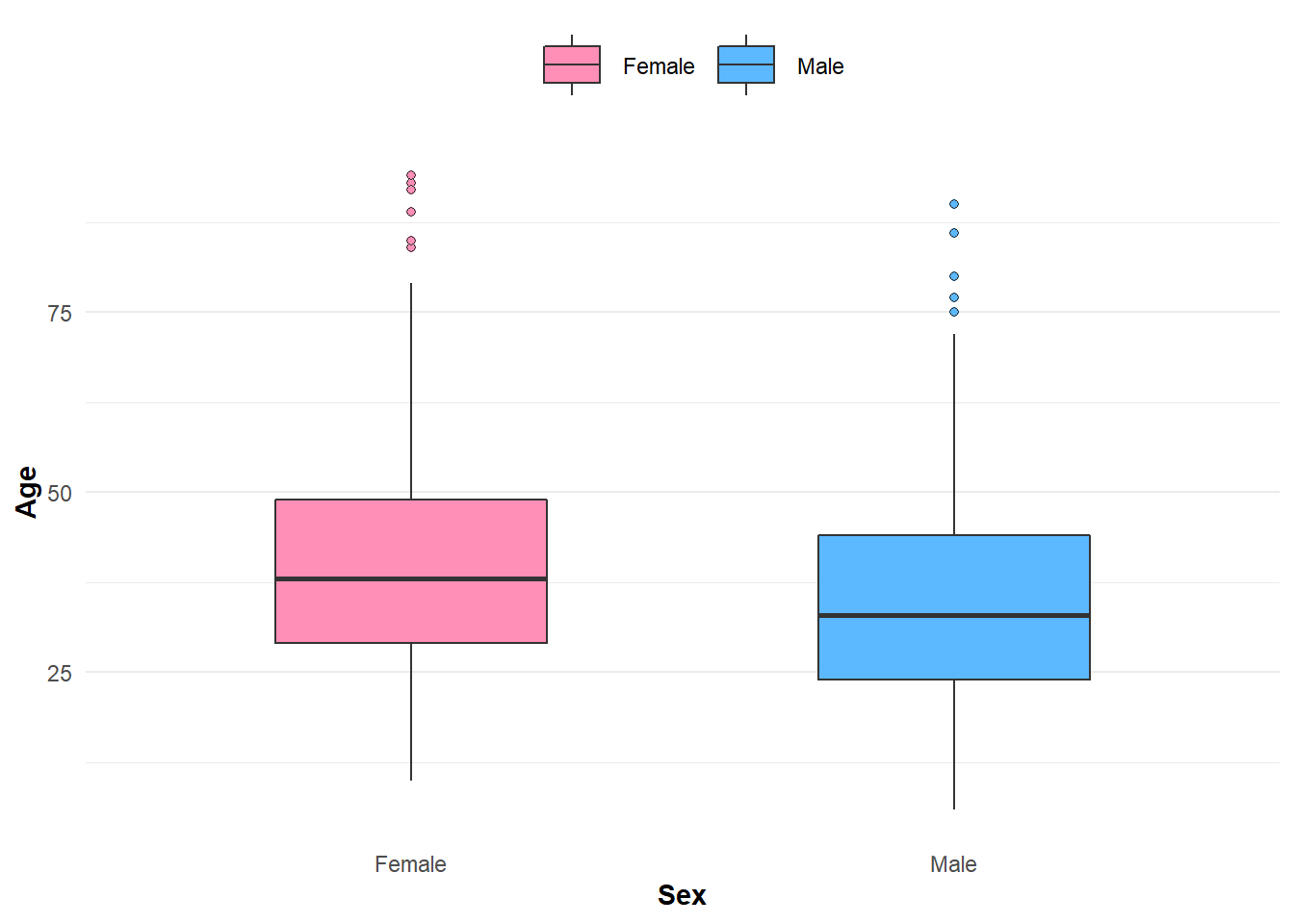
Figure 2: Distribution of disease by age and sex.
We could plot each variable against the outcome (disease) separately but since the data has just 4 variables it is possible to observe the relationships at the same time. This may not be always preferable, as the visualization can become quite dense; that is to say, it could be hard to digest all of the dimensions presented from the data. How the variables are assigned to plot are important for aiding interpretation. As our interest is the presence/absence of Disease X, we assign this variable as the plot color to ensure it is included in each panel. In this instance plotting all the variables does provide some interesting insights:
- Males appear to have a larger representation in the younger age groups
- Disease is present in higher proportions among older age groups
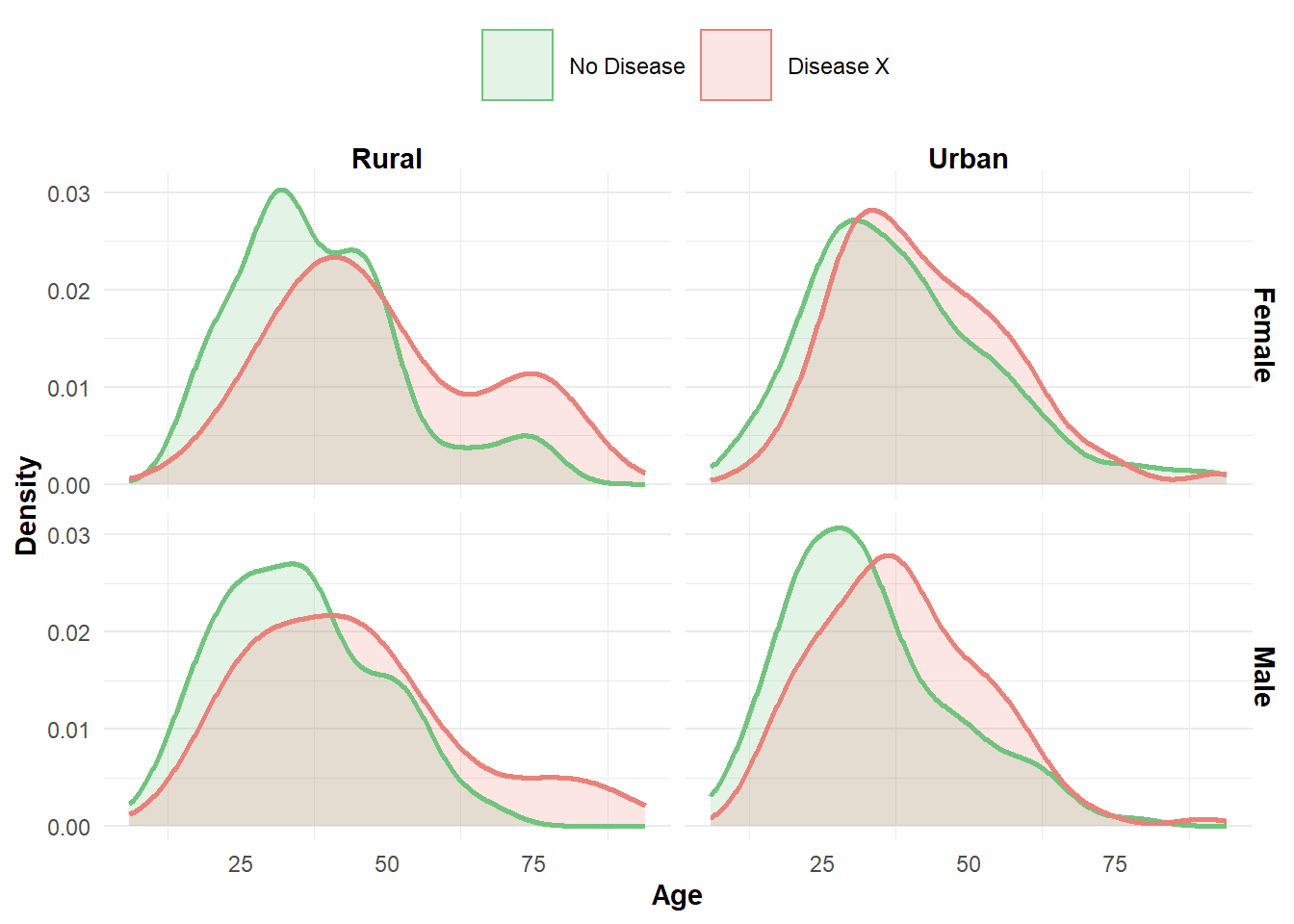
Figure 3: Disease X in terms of age, sex, and location.
Although I used a density plot in the example above, some may prefer using a box-plot as a suitable alternative.
Age seems to have a strong impact on the disease outcome which may be masking more subtle relationships. When we remove age we observe urban areas have a higher proportion of Disease X, and there is subtle evidence of a higher proportion of disease among females. None of this should come as a surprise, as we set these relationships in advance but it is nice to validate them through these figures.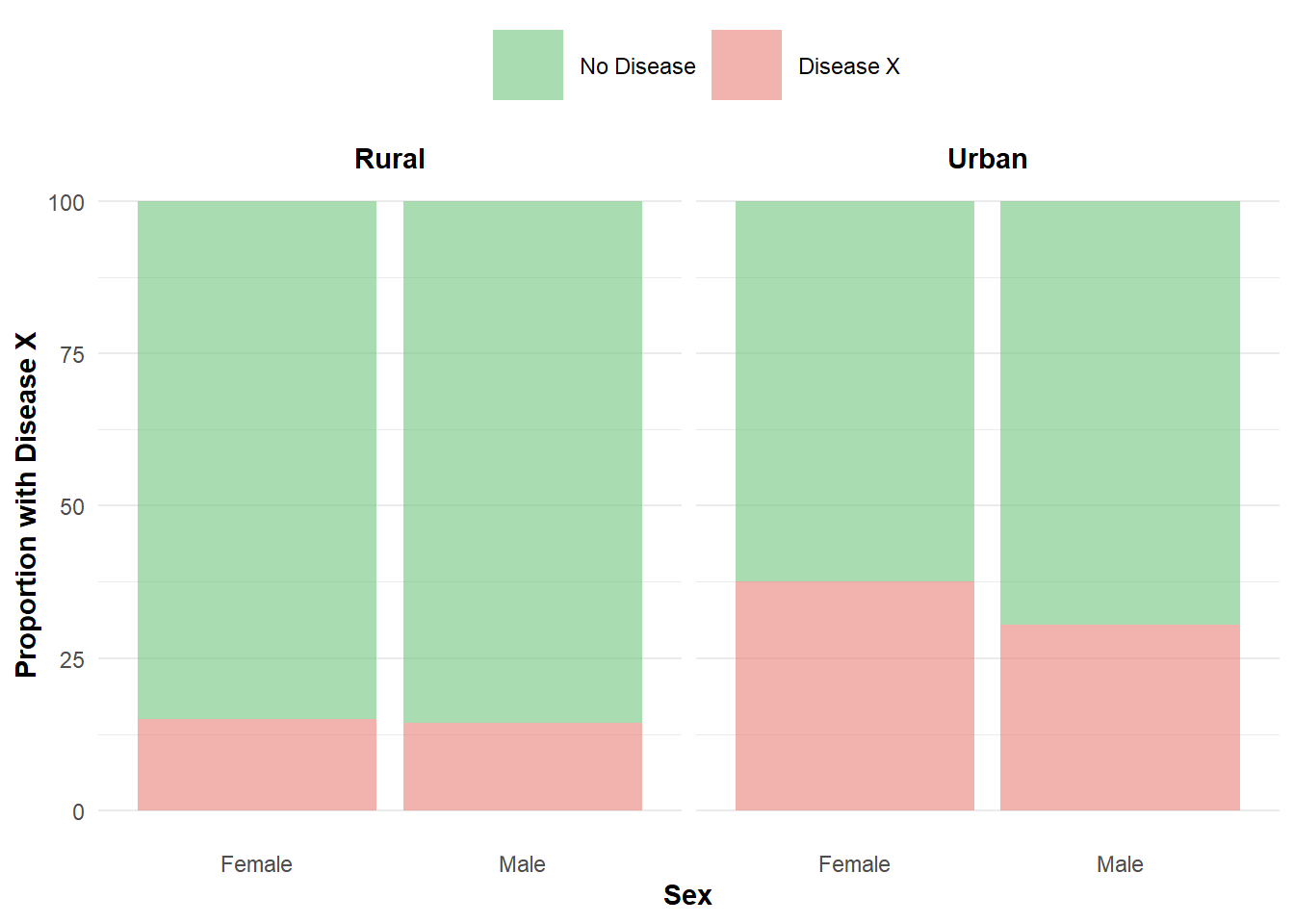
Figure 4: Proportion of Disease X in terms of sex and location.
A case for simulated data
You may be asking yourself, why would I bother ‘making up’ data, it seems like a lot of trouble? It even may appear to reinforce bias as the data is often a product from our own assumptions. However, in reality, simulated data have a great amount of value, here are just a few examples:
- Simulation allows us to know the exact data generation process, an important tool to troubleshoot statistical models and see where they succeed or fail.
- Creating ‘What-If’ scenarios can provide valuable insight for program and policy planning.
- Although there are many publicly-available datasets in our digital age, many are highly aggregated, difficult to link to other important sources, and hard to access when content is highly sensitive (e.g. health records)
Focusing on the last point, it can be very difficult to access and share interesting data in public health. For example, most sources that share infectious disease information have limited content to reduce the chance of identifying individuals. Sometimes there isn’t even enough information available to do basic descriptive epidemiology, which usually requires key demographics (e.g. age, sex), locations (e.g. urban/rural, health authority), and time (e.g. diagnosis date, treatment administration date). Obviously, this can raise concerns about privacy. For meaningful and interesting analyses this type of information is needed and to obtain access a data-sharing agreement and ethical approval is often required. In academic research endeavors this is a necessity but for this website I resort to real data where it is openly available and simulated data when it is not. When the focus is to showcase specific methods, simulated data is all we really need. Even common problems that plague ‘real’ data, such as missing information, can be added to our simulated data.
Simulation toolbox
Agreeing on the usefulness of simulating data, how can it be done? There are many approaches with varying complexity:
- Agent/individual-based models
- Random variables simulated from probability distributions
- Creating Bayesian networks based upon priors and/or learned from data
Most approaches are available in R or its host of packages, albeit with a tradeoff between flexibility and complexity. For instance, NetLogo is a programming environment for agent-based simulation and can connect to R through the RNetLogo package; this however still requires knowledge of the NetLogo syntax. Other simulation approaches in R are available from HydeNet, greta, RStan, and simstudy. Some packages are limited as they only allow certain data types (e.g. discrete or continuous) and the possible relationships that can exist between them (e.g. linear trend). Typically, ‘low-level’ interfaces (i.e. a package that gets you close to the ‘engine’) allow more freedom but increase the learning curve and chances of blunder. Furthermore, a selection of methods listed require data to operate and for some purposes this may be unsuitable.
I am partial to Bayesian networks, which is my method of choice in this post, as I find their associated diagrams a powerful visualization tool to understand the model. They can also be created from our imagination, or trained on any available data we happen to have. Flexible and powerful!
Basic simulation example
Before I continue to explain the method I used to create Bayes’ Town, now is a good time to demonstrate that simulation techniques are not out of anyone’s reach.
Keeping with the theme of health, let’s simulate the probability of death by boredom in Bayes’ Town. Hopefully you are not suffering from this affliction as it is quite serious, as we will soon discover.
As a binary outcome, we can use the binomial distribution for modeling death. The probability of death will be a function of an intercept term and the binary explanatory variable for ‘boredom’ (0: not bored, 1: bored). The logit link will map the linear combination of the intercept and ‘boredom’ term between 0% and 100% probability. In math jargon this looks like:
\[\begin{align*} & y_i \sim Binomial(n, p_i) \\ & logit(p_i) = \alpha + \beta x_i\\ \end{align*}\]

If you are like me, you may get nervous when a page becomes overtaken by formulae. I promise, it is not as bad as it looks. I usually feel more at ease once I see the formulae translated to code, which we will do now.
# Set 100,000 people in our population
n <- 1e5

# Half of our population is bored
bored <- rep(c(0,1), each = n/2)

# Bored has a small increase to the log-odds of death
beta <- 0.3

# The baseline chance of death is low
alpha <- 0.05

# The log-odds of the outcome (arithmetic from the formula above!)
logodds <- alpha + beta * bored

# Probability of death (size = 1, only one death possible per person!)
death_probability <- rbinom(n, prob = plogis(logodds), size = 1)

# Final dataset
data <- data.frame(boredom = bored,
                   death = death_probability)
We can see a relationship between boredom and death in a simple 2x2 table. The values on the bottom of the table compare the odds of not being bored among the living and dead; these results show a 1.4x higher odds of death among those experiencing boredom.
library(knitr)
library(kableExtra)

# Function to calculate odds
odds <- function(x) round(x[[1]]/x[[2]], 3)

# Create table with odds, adjust rounding, and format
summary_tbl <- table(Boredom = data$boredom,
                     Death = data$death) %>%
  addmargins(margin = c(1,2),
             FUN = list(Odds = odds),
             quiet = T)

summary_tbl[c(1:3), c(1,3)] <- as.character(summary_tbl[c(1:3), c(1,3)])

summary_tbl %>%
  kable(caption = 'Relationship between boredom and death.') %>%
  kable_styling(full_width = T) %>%
  pack_rows('Boredom', 1,2, label_row_css = 'border-bottom:0px solid;') %>%
  add_header_above(c(" ", "Death" = 3), align = 'l') %>%
scroll_box(box_css = "", extra_css = 'overflow-x: auto; width: 100%')| 0 | 1 | Odds | |
|---|---|---|---|
| Boredom | |||
| 0 | 24481 | 25519 | 0.959 |
| 1 | 20749 | 29251 | 0.709 |
| Odds | 1.18 | 0.872 | 1.353 |
If that isn’t enough to convince you that the simulated data created a positive correlation between boredom and death, let’s pass the data through a logisitic regression model to see how well we can retrieve the original parameters for the intercept (0.05) and beta term (0.3).
coef(glm(death ~ boredom, data = data, family = 'binomial')) %>%
  round(3) %>%
  kable(col.names = 'Estimate', caption = 'Parameter estimates for model on boredom and death.') %>%
  kable_styling() %>%
  scroll_box(box_css = "",
extra_css = 'overflow-x: auto; width: 50%')| Estimate | |
|---|---|
| (Intercept) | 0.042 |
| boredom | 0.302 |
That is pretty close! We could take this simulation further and create a dependency of boredom upon additional terms. I encourage you to explore other situations, such as collinear variables. As the simulation becomes increasingly complex other approaches may be easier to maintain. This is what we will discuss next.
Data simulation with Bayesian networks
Another approach to simulate data is using BNs, specifically hybrid BNs which are more complex but allow the use of both continuous and discrete variables. Although raw data are typically included in these models, it is also possible to create BNs based solely on our own conceptions. In this case, we can say we are creating a network using prior probability distributions.
Up until now we have focused on the outputs from the data simulation in hopes of showcasing its capabilities without yet being cowed in either boredom or fear from maths. For those willing, understanding the details will curb the feeling of mathematical mysticism and avoid ascribing too much faith in the simulation and underlying model. Although there are many strategies to simulate data, in this example I have used a Bayesian Network (BN), known by several other names, including the less exciting, directed graphical model. The overall idea is simple:
- First create a relationship using a graph, consisting of nodes and arcs. Each node represents a random variable (e.g. age, sex) and their arcs define relationships. Mathematically, this is typically seen as: \(G = (X, A)\), where \(X\) is a set of variables.
- Next, we assign probability distributions to the variables. BNs are useful as they can describe the global probabilistic relationship among \(X\) by their various local distributions. That is to say, we understand the probability of every node by the relationship it has to its direct parent nodes. Again, as Greek soup this is seen as: \(Pr\mathbf(X) = \prod_{i=1}^{p}Pr(X{_i}|\textstyle\prod_{X_i})\).
When we know both the graph as well as the local distribution, the model is called an expert system. In other words, everything is defined upfront by us; we aren’t using any data to directly fit the model. In Bayesian lingo, we are essentially making a model with just priors.

If you feel overwhelmed do not fret, I felt this way initially too (and perhaps still do). Deeper understanding comes at a cost. Fortunately, half of our job is already done as we have previously defined the graph using our infinite wisdom. Now we just need to decide on the probability distributions and how they relate between each node.
Model definition
Similar to our simple example, we will start by assigning our parameter priors, essentially a set of distributions for the intercept and coefficient terms in the model.
\[ \begin{align*} & \textbf{Prior parameters}\\ & a_{disease} \sim Normal(-10, 10) \\ & b_{age} \sim Normal(0.015, 10) \\ & b_{sex} \sim Normal(0.005, 10) \\ & b_{urbanity} \sim Normal(5, 10) \\ \\ \end{align*} \] \(a_{disease}\) is the baseline odds of disease and the other parameters define the magnitude by which they increase the odds of disease. Next, we create distributions for our variables of interest (alternatively, these could be set as fixed values).
\[ \begin{align*} & \textbf{Random variable priors}\\ & sex \sim Binom(propMale, 1) \\ & urbanRural \sim Binom(0.8, 1) \\ & \begin{aligned} age \sim Gamma((age_{shape} + &age\_param * sex),\\ 1/age_{scale}) \end{aligned}\\ \\ \end{align*} \]
We also will have several input parameters for our variables. We can adjust these or the prior parameters to create strong/weaker, or entirely different, relationships.
\[ \begin{align*} & \textbf{Input parameters}\\ & propMale = 0.52 \\ & age_{shape} = 6 \\ & age_{scale} = 6 \\ & age\_param = 0.7 \\ \\ \end{align*} \]
And finally, we need to assign a likelihood function for the prior predictive simulation. This is the distribution for Disease X based upon the relationship of age, sex, and location.
\[ \begin{align*} & \textbf{Likelihood function}\\ & disease \sim Binom(p, 1) \\ & \begin{aligned} logit(p) &= a_{disease} \\ &+ b_{age}(age) \\ &+ b_{sex}(sex) \\ &+ b_{urbanity}(urbanRural)\\\\ \end{aligned} \end{align*} \]
These formulae may look confusing, but they are outlining very similar concepts to the simple example between boredom and death. If you are a little lost, the DAG from the beginning should help. In plain English we are saying that:
- Sex is slightly more likely to be male
- Location has a much higher chance to be urban
- Age is slightly dependent upon sex; females reach slightly older age groups on average
- Disease X is a linear relationship between age, sex, and location
- The strength of age, sex, and location are pulled from a distribution of values that we can tweak to increase/decrease their strength.
In R code it looks quite similar:
# Set input parameters (could be included directly in the model below if we arent changing often)
inputParam <- list(p_sex = 0.52,
                   age_shape = 6,
                   age_scale = 6,
                   age_param = 0.7)

# Define model (character string is code for JAGS)
simModel <-  as.character('
                      model {
                        a_disease ~ dnorm(-10, 10);
                        b_age ~ dnorm(.015, 10);
                        b_sex ~ dnorm(.005, 10);
                        b_urbanity ~ dnorm(5, 10);

                        sex ~ dbinom(p_sex, 1);
                        urbanRural ~ dbinom(0.8, 1);
                        age ~ dgamma((age_shape + age_param * sex), 1/age_scale);

                        logit(p) <- a_disease + b_age * age + b_sex * sex + b_urbanity * urbanRural;
                        disease ~ dbinom(p, 1);
                      }')
This is the set of rules that governs Bayes’ Town citizens. Right now it provides a single snapshot but it is possible to extend this to a dynamic BN to create multiple time slices.
Bayes’ Theorem is used to solve this type of question and the equation may look simple enough… \[P(A|B) = \frac{P(B|A)P(A)}{P(B)}\] I do not provide details here as there are a plethora of resources online that go through Bayes’ Theorem; however, I will point out that a special ‘engine’ is often required to solve these models. When the distributions are complex, the solutions become non-trivial. Whilst some examples such as the beta-binomial have closed-form solutions, others require special sampling methods to solve, which we will discuss next.
MCMC and rjags
With the rules defined to create Disease X in Bayes’ Town, we now need to perform the simulation. The procedure used is called markov chain monte carlo (MCMC), a stochastic method to estimate posterior probability distributions. In short this means we collect samples of possible parameter values instead of attempting to directly compute them. The results are then understood in terms of their sample distribution. However, generating these samples is not always easy and there are various MCMC methods to tackle this challenge, albeit with their own limitations and trade-offs.
1. Metropolis algorithm: original and ‘simple’ MCMC implementation.
2. Metropolis-Hastings algorithm: an extension to the metropolis algorithm.
3. Gibbs sampling: more efficient sampling by using adaptive proposals (BUGS and JAGS software use this method).
4. Hamiltonian Monte Carlo (HMC): runs a (resource expensive) physics simulation to generate informative samples. HMC provides useful diagnostics but currently cannot sample discrete parameters (not easily at least). STAN uses this method and is considered harder to learn than BUGS.
Numerous R packages implement the assortment of MCMC methods but require, or are built on top of, an R interface to STAN (e.g. rstan) or JAGS (e.g. rjags). For my current purposes, I decided to use rjags (authored by Martyn Plummer who is also the creator of JAGS) since it can generate discrete values and follows a syntax similar to R. Using rjags directly is a bit more complex (as we saw in the model definitions) but provides flexibility and customization.
There are three steps to run a model with JAGS: (1) Define, (2) Compile, and (3) Simulate. We have already done the first step, for the rest I created helper functions to pass the model to JAGS and retrieve the samples! This may be unnecessary but I found it to be a helpful abstraction. We can always dip into rjags if we need something more specific.
The R6 package was used to encapsulate the BayesTown object created from the simulation. This object is created by running BayesTown$new() with the provided model (simModel) and input parameters (inputParam). JAGS will then compile and perform the simulation, returning the results to the assigned object class. A subset of variables can be retained via the set_variables() method and a new draw can be done via resample(). Various diagnostics are also accessible. If this is still a bit unclear, the complete example in the next section may be of help.
Full simulation run
At the beginning a model and parameters were already determined. Below I provide the code to create the simulated Bayes’ Town. A few helper functions built on top of rjags make the process a bit more friendly to read. The Bayes’ Town example is an expert system using just priors but if we decide to include data in the model we simply add a loop to the likelihood function.
# Set input parameters
inputParam <- list(p_sex = 0.52,
                   age_shape = 6,
                   age_scale = 6,
                   age_param = 0.7)

# Define model
simModel <-  as.character('
                      model {
                        a_disease ~ dnorm(-10, 10);
                        b_age ~ dnorm(.015, 10);
                        b_sex ~ dnorm(.005, 10);
                        b_urbanity ~ dnorm(5, 10);

                        sex ~ dbinom(p_sex, 1);
                        urbanRural ~ dbinom(0.8, 1);
                        age ~ dgamma((age_shape + age_param * sex), 1/age_scale);

                        logit(p) <- a_disease + b_age * age + b_sex * sex + b_urbanity * urbanRural;
                        disease ~ dbinom(p, 1);
                      }')

# Simulate new town
newTown <- BayesTown$new(population_size = 1000,
                      jags_data = inputParam,
                      n.chains = 2,
                      n.iter = 5000,
                      jags_model = simModel)

# Keep only subset of parameters of interest
newTown$set_variables(c('age', 'sex', 'urbanRural', 'disease'), mode = 'include')

# Resample data
newTown$resample()
We can now use newTown as we saw at the start of the post and explore our newly simulated dataset!
Resources
Useful data sources
Software and details on simulation methods
Information on Bayesian statistics
While there are many blogs and online articles about Bayesian statistics and Bayesian networks, I found books were my best resource; enjoyable and worth the price tag.
- Statistical Rethinking and related YouTube channel
- Bayesian Networks with Examples in R
- Bayesian Networks without Tears, a great introduction to the topic.
Allen O'Brien
Infectious Disease Epidemiologist
I am an epidemiologist with a passion for teaching and all things data.