Tokyo Ramen: Mapping with OpenStreetMaps

Load packages

The three core packages used here are ggplot2, sf, and osmdata as they are integral to the mapping components. These all appear to be stable and work nicely together. They are also all under active development. Although several other packages could be swapped out to one’s own preference, I have selected primarily tidyverse packages.

# Packages to make data munging easier...
library('magrittr')
library('stringr')
library('dplyr')
library('tidyr')
library('scales')

# Packages for fancy maps...
library('sf')
library('ggplot2')
library('osmdata')

Create bounding box

As our goal is to map Tokyo ramen sellers, we first need to create a bounding-box specific to this location. There are two main ways this can be performed. First, we can use the getbb() function from osmdata which returns a vector of lat/long coordinates. However, I found this less than ideal for Greater Tokyo as the shape, which includes several islands in the pacific, is not well defined by default bounding-box. In essence, the bounding box is too large, and I only had interest in the Tokyo core. Instead I used the second more manual method of defining the bounding box myself using an online tool from OSM. I then passed the coordinates to the bbox parameters of opq() which will query OSM for features in that defined area.

# Manually define the bounding-box for Tokyo core
loc_boundary <- c(139.6867, 35.6238, 139.8642, 35.7643)

Query OSM for map features

Now that we have Tokyo’s coordinates, we can use that to pull out select geographic features. This works by providing key-value pairs to the add_osm_feature() function which will translate the input to an overpass API query. This abstraction is welcome as the overpass query syntax is not easily picked up in an afternoon. If you want to see the actual overpass query you can extract the string using opq_string(). You can also observe available values for a particular feature key using available_tags(). After some trial and error you’ll know which values you want in your map.

After digging through the available features, we’ll extract those for the major highways and convert them to an sf object. The request may fail on the first attempt to query the server, but should work on the second or third attempt.

# Large roads
large_roads <- opq(loc_boundary) %>% 
  add_osm_feature(key = "highway", 
                  value = c("motorway", "primary", "secondary",'tertiary')) %>%
  osmdata_sf

Let’s see what this looks like using ggplot2. This should be easy with geom_sf() since we already converted the OSM data into an sf object. Depending on the feature, the information needed to map will be stored in various formats; for roads, this is typically as lines, but multilines, points, and polygons are also possible depending on the feature selected.

# Create ggplot and add road layer
tokyo_ramen <- ggplot() +
  geom_sf(data = large_roads$osm_lines)

tokyo_ramen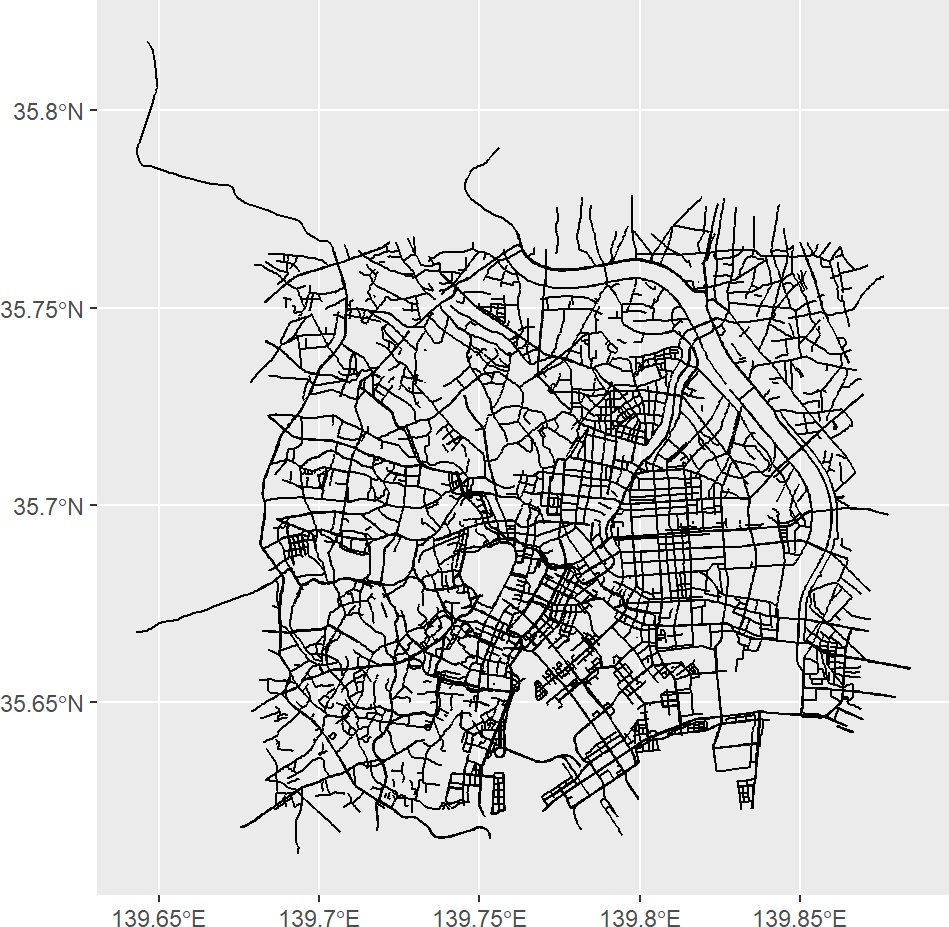

Building on this, we can now add smaller roads to see the complexity of Tokyo’s criss-crossed concrete landscape…

# Small roads query
small_roads <- opq(loc_boundary) %>% 
  add_osm_feature(key = "highway", 
                  value = c('unclassified', 'residential', "service")) %>%
  osmdata_sf

# Add to plot
tokyo_ramen <- tokyo_ramen +
  geom_sf(data = small_roads$osm_lines)

As a bay city, there are also many waterways in Tokyo which can also be accessed through OSM. A mixture of both osm_lines and osm_polygons are needed in this case. Let’s add those as well…

# Small waterways
waterway <- opq(loc_boundary) %>% 
  add_osm_feature(key = 'waterway',
                  value = c('canal')) %>%
  osmdata_sf

# Small rivers and banks (lines)
waterway_river <- opq(loc_boundary) %>% 
  add_osm_feature(key = 'waterway',
                  value = c('river', 'riverbank')) %>%
  osmdata_sf

# Polygons for rivers (query is chained for 'and' operation)
waterbody <- opq(loc_boundary) %>% 
  add_osm_feature(key = 'natural',
                  value = c('water')) %>%
  add_osm_feature(key = 'water',
                  value = c('river')) %>%
  osmdata_sf 

# Add to plot
tokyo_ramen <- tokyo_ramen +
  geom_sf(data = waterway$osm_lines) +
  geom_sf(data = waterway_river$osm_lines) +
  geom_sf(data = waterbody$osm_polygons)

tokyo_ramen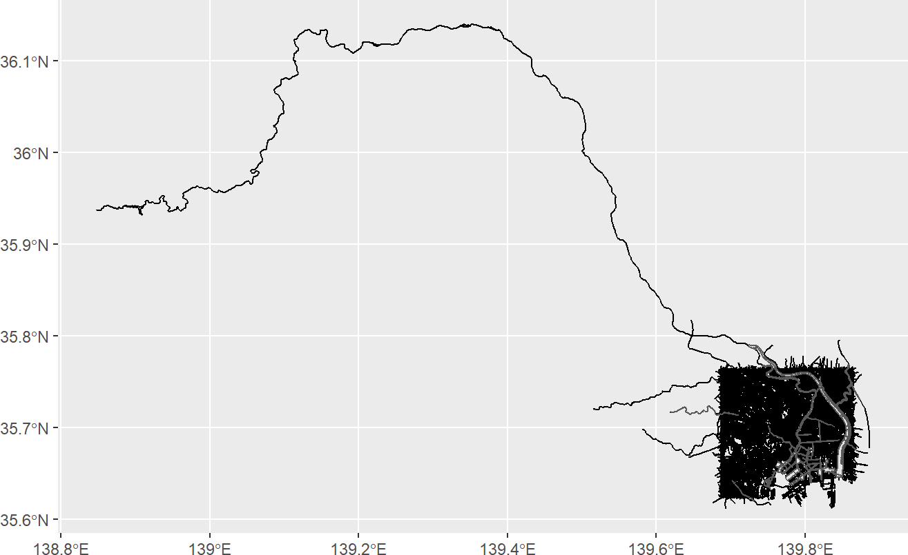

At this point, we have a truly ugly blob of features and the waterways have extended beyond the Tokyo core…

So, let’s start some of the formatting to make this a bit more visually pleasing. Since each feature has its own layer it is easy to customize each to our liking. To ensure aes() elements are not inherited, we set it to FALSE in each geom_sf().

# Define colors
colour_water <- "#5cbef4"
colour_large_road <- "#b8ab66"
colour_small_road <- "#766759"

# Ensure bounding box is maintained
tokyo_ramen <- ggplot() +
  xlim(loc_boundary[c(1,3)]) +
  ylim(loc_boundary[c(2,4)])

# Format feature layers
tokyo_ramen <- tokyo_ramen +  
  geom_sf(data = waterway$osm_lines,
          color = colour_water,
          size = 1, 
          inherit.aes = F) +
  geom_sf(data = waterway_river$osm_lines,
          color = colour_water,
          inherit.aes = F) +
  geom_sf(data = waterbody$osm_polygons,
          color = colour_water,
          fill = colour_water,
          inherit.aes = F) +
  geom_sf(data = large_roads$osm_lines,
          color = colour_large_road,
          size = .25,
          alpha = .8,
          inherit.aes = F)+
  geom_sf(data = small_roads$osm_lines,
          color = colour_small_road,
          size = .05,
          alpha = 0.1,
          inherit.aes = F)

# Adjust the overall theme, add custom changes
tokyo_ramen <- tokyo_ramen +  
  theme_minimal() +
  theme(plot.background = element_rect(fill = "#282828"),
        axis.text = element_blank(),
        axis.ticks = element_blank(),
        axis.title = element_blank(),
        axis.line = element_blank(),
        panel.grid = element_blank())

tokyo_ramen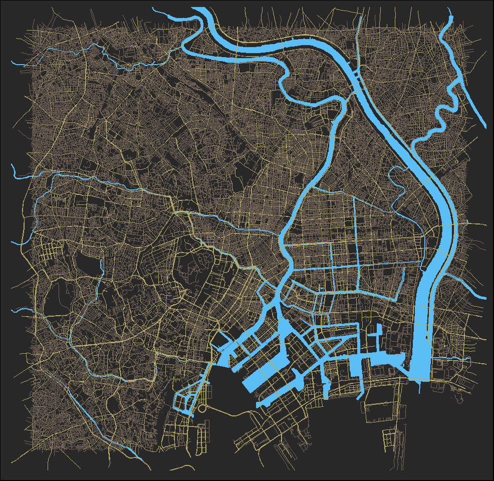

This is looking much better but there is one glaring feature missing, the water for the coastline in the bottom right of the map. This is a bit trickier than simply adding a feature from OSM. The coastline feature has a line format and will not create a complete polygon to represent the body of water. Thankfully, there are some solutions readily available to us online, such as one outlined by Florian Zenoni. The st package provides several functions such as st_line_merge() and st_cast() to accomplish this.

# Coastline will help fill the area in the bay
coastline <- opq(loc_boundary) %>% 
  add_osm_feature(key = 'natural',
                  value = c('coastline')) %>%
  osmdata_sf

# Convert `line` to `multilines`, and then convert to a `polygon`
coastline <- coastline$osm_lines %>% st_union %>% st_line_merge() %>% sf::st_cast('POLYGON')

# Add to map
tokyo_ramen <- tokyo_ramen +
    geom_sf(data = coastline,
          fill = colour_water,
          color = colour_water,
          inherit.aes = F)

# Make sure roads are on top!
tokyo_ramen <- tokyo_ramen +
  geom_sf(data = large_roads$osm_lines,
          color = colour_large_road,
          size = .25,
          alpha = .8,
          inherit.aes = F)+
  geom_sf(data = small_roads$osm_lines,
          color = colour_small_road,
          size = .05,
          alpha = 0.1,
          inherit.aes = F)

tokyo_ramen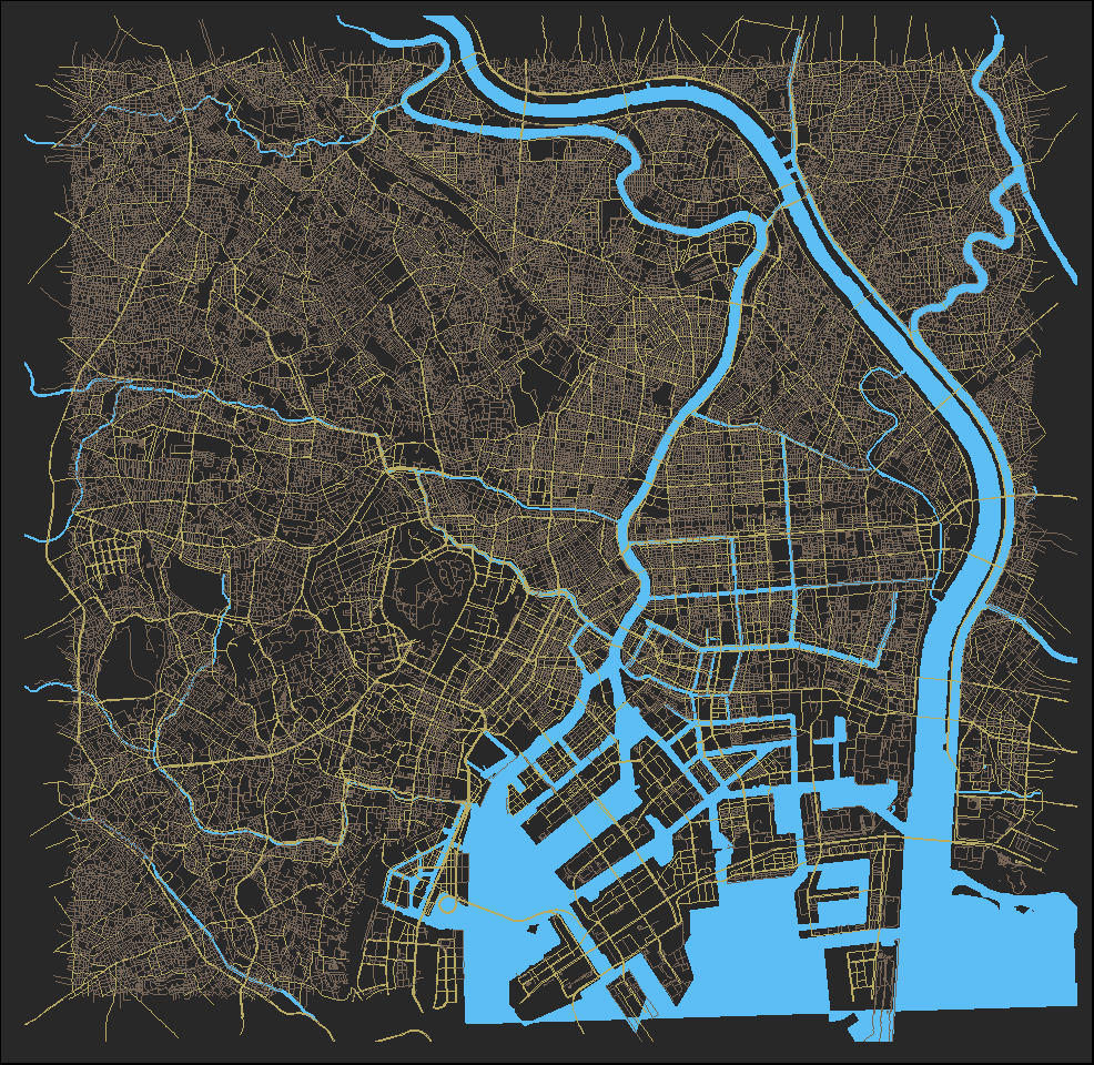

Superimposing ramen data

Our base-map is looking good but, as pretty as it looks, it doesn’t tell me anything about ramen. After exploring available OSM features, there is one under amenity for restaurants. With a bit of basic string manipulation we can pull out all restaurants that have the mention of ramen. Using their coordinates, we create a dataset of these points we bin and plot them into square tiles using geom_bing2d(). After some minor fiddling with the scale features, formatting, and tightening the margins with coord_sf(), we finally see the density of ramen shops!

# Grab features for restaurants
restaurant <- opq(loc_boundary) %>% 
  add_osm_feature(key = 'amenity',value =   'restaurant') %>%
  osmdata_sf

# Grab all points that feature the word 'ramen'.
ramen <- restaurant$osm_points %>% 
  mutate(cuisine = str_to_lower(str_trim(cuisine))) %>%
  filter(str_detect(cuisine, 'ramen')) %>%
  select(geometry, cuisine)

# Create a dataset for all the ramen points and their coordinates
ramen <- ramen %>% 
  as_tibble() %>%
  mutate(id = names(geometry)) %>%
  unnest('geometry') %>% 
  group_by(id) %>%
  mutate(coord = c('long', 'lat')) %>%
  pivot_wider(names_from = coord, values_from = geometry)

# Add to map
tokyo_ramen <- tokyo_ramen +
  geom_bin2d(data = ramen, aes(x = long, y = lat), color = 'white', alpha = 0.9) +
  scale_fill_gradient(low = 'white',
                      high =  '#d25050', 
                      breaks = pretty_breaks(),
                      guide = guide_colourbar(title = 'Ramen shops', 
                                              title.position ="top",
                                              ticks.colour = 'transparent',
                                              title.theme = element_text(color = 'snow1', face = 'bold'),
                                              label.theme = element_text(color = 'snow1', face = 'bold', size = 10),
                                              label.position = 'bottom',
                                              direction = 'horizontal', 
                                              title.hjust = 0.5,
                                              barwidth = 10, barheight = 0.55)) +
  theme(legend.position = 'bottom',
        legend.box = 'horizontal',
        legend.box.margin = margin(t = 15)) +
  coord_sf(expand = F)

tokyo_ramen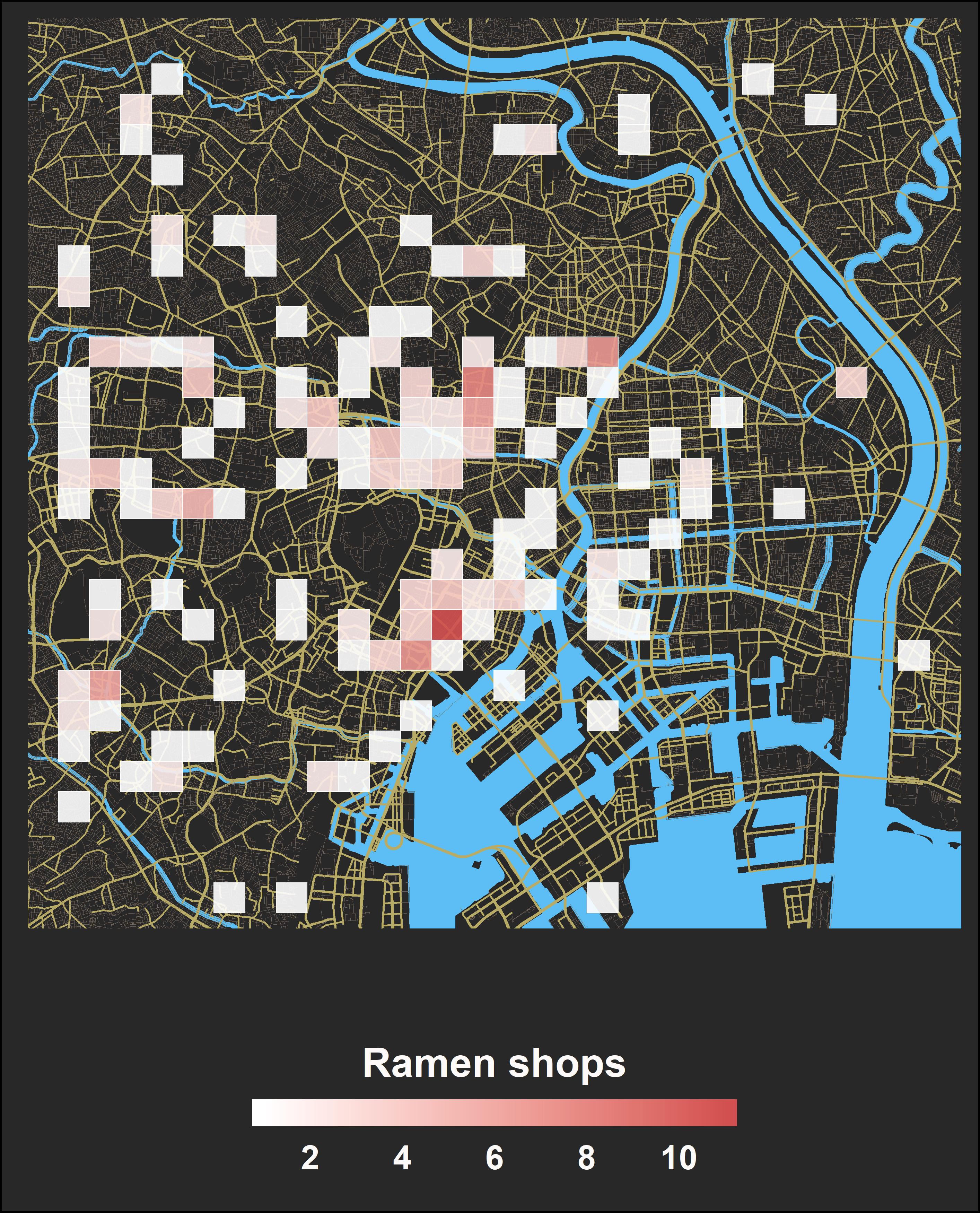

Now, the first thing one may think when they see this complete map is: “that seems to be fewer shops than I would expect”. And I believe you would be right. In 2016, there were an estimated 10,000 ramen shops in Japan, many of which I would expect to be in the Tokyo core. As such, this brings into question the quality of the amenity data available in OSM. After a quick search, OSM data has been known to suffer from several biases, one of which must include a rather incomplete source of restaurant locations. Although there may be better alternative data-sources, I think this map provides a good sense of what we aimed to accomplish, with some room for improvement.

All together now…

For convenience, the code below is the complete set required to recreate the map with superimposed ramen shop density. Although I am sure the formatting and styling could be taken even further, I think it is good for now.

#---------------------#
# Setup
#---------------------#

# Packages to make data munging easier...
library('magrittr')
library('stringr')
library('dplyr')
library('tidyr')
library('scales')

# Packages for fancy maps...
library('sf')
library('ggplot2')
library('osmdata')

# Manually define the bounding-box for Tokyo core
loc_boundary <- c(139.6867, 35.6238, 139.8642, 35.7643)

# Define colors
colour_water <- "#5cbef4"
colour_large_road <- "#b8ab66"
colour_small_road <- "#766759"


#---------------------#
# Query OSM
#---------------------#

# Large roads
large_roads <- opq(loc_boundary) %>% 
  add_osm_feature(key = "highway", 
                  value = c("motorway", "primary", "secondary",'tertiary')) %>%
  osmdata_sf

# Small roads query
small_roads <- opq(loc_boundary) %>% 
  add_osm_feature(key = "highway", 
                  value = c('unclassified', 'residential', "service")) %>%
  osmdata_sf

# Small waterways
waterway <- opq(loc_boundary) %>% 
  add_osm_feature(key = 'waterway',
                  value = c('canal')) %>%
  osmdata_sf

# Small rivers and banks (lines)
waterway_river <- opq(loc_boundary) %>% 
  add_osm_feature(key = 'waterway',
                  value = c('river', 'riverbank')) %>%
  osmdata_sf

# Polygons for rivers (query is chained for 'and' operation)
waterbody <- opq(loc_boundary) %>% 
  add_osm_feature(key = 'natural',
                  value = c('water')) %>%
  add_osm_feature(key = 'water',
                  value = c('river')) %>%
  osmdata_sf 

# Coastline will help fill the area in the bay
coastline <- opq(loc_boundary) %>% 
  add_osm_feature(key = 'natural',
                  value = c('coastline')) %>%
  osmdata_sf

# Convert `line` to `multilines`, and then convert to a `polygon`
coastline <- coastline$osm_lines %>% st_union %>% st_line_merge() %>% sf::st_cast('POLYGON')

# Grab features for restaurants
restaurant <- opq(loc_boundary) %>% 
  add_osm_feature(key = 'amenity',value =   'restaurant' ) %>%
  osmdata_sf


#---------------------#
# Ramen dataset
#---------------------#

# Grab all points that feature the word 'ramen'.
ramen <- restaurant$osm_points %>% 
  mutate(cuisine = str_to_lower(str_trim(cuisine))) %>%
  filter(str_detect(cuisine, 'ramen')) %>%
  select(geometry, cuisine)

# Create a dataset for all the ramen points and their coordinates
ramen <- ramen %>% 
  as_tibble() %>%
  mutate(id = names(geometry)) %>%
  unnest('geometry') %>% 
  group_by(id) %>%
  mutate(coord = c('long', 'lat')) %>%
  pivot_wider(names_from = coord, values_from = geometry)


#---------------------#
# Create map
#---------------------#

# Ensure bounding box is maintained
tokyo_ramen <- ggplot() +
  xlim(loc_boundary[c(1,3)]) +
  ylim(loc_boundary[c(2,4)])

# Add and format feature layers
tokyo_ramen <- tokyo_ramen + 
  geom_sf(data = waterway$osm_lines,
          color = colour_water,
          size = 1, 
          inherit.aes = F) +
  geom_sf(data = waterway_river$osm_lines,
          color = colour_water,
          inherit.aes = F) +
  geom_sf(data = waterbody$osm_polygons,
          color = colour_water,
          fill = colour_water,
          inherit.aes = F) +
  geom_sf(data = coastline,
          fill = colour_water,
          color = colour_water,
          inherit.aes = F) +
  geom_sf(data = large_roads$osm_lines,
          color = colour_large_road,
          size = .25,
          alpha = .8,
          inherit.aes = F) +
  geom_sf(data = small_roads$osm_lines,
          color = colour_small_road,
          size = .05,
          alpha = 0.1,
          inherit.aes = F)

# Add the ramen shops
tokyo_ramen <- tokyo_ramen +
  geom_bin2d(data = ramen, aes(x = long, y = lat), color = 'white', alpha = 0.9) +
  scale_fill_gradient(low = 'white',
                      high =  '#d25050', 
                      breaks= pretty_breaks(),
                      guide = guide_colourbar(title = 'Ramen shops', 
                                              title.position ="top",
                                              ticks.colour = 'transparent',
                                              title.theme = element_text(color = 'snow1', face = 'bold'),
                                              label.theme = element_text(color = 'snow1', face = 'bold', size = 10),
                                              label.position = 'bottom',
                                              direction = 'horizontal', 
                                              title.hjust = 0.5,
                                              barwidth = 10, barheight = 0.55))

# Adjust theme
tokyo_ramen <- tokyo_ramen +
  theme_minimal() +
  theme(plot.background = element_rect(fill = '#282828'),
        axis.text = element_blank(),
        axis.ticks = element_blank(),
        axis.title = element_blank(),
        axis.line = element_blank(),
        panel.grid = element_blank(),
        legend.position = 'bottom',
        legend.box = 'horizontal',
        legend.box.margin = margin(t = 15)) +
  coord_sf(expand = F)